Finding the dominant colors of an image
Posted on Tue 24 July 2018 in OpenCV
The typical way to isolate or find an object in an image is to look for its color. You specify a range of colors, then use OpenCV to identify regions in an image that contain colors within that range. But, even if you know the exact color of your target, lighting, shadows, and your camera's sensor will alter the detected color. So, how do you best determine the color range to use?
In this article, I'll explore some different methods to work with colors. In a future article, we'll use this knowledge, plus selecting a region of interest within an image/video to determine the exact range of colors needed to isolate an object.
Let's say your goal is to isolate the puppy in this image. You'll notice that his fur color varies between an off-white to a golden tan. The foreground is brighter, making his hindquarters darker and less richly colored. The toy he has is only a bit darker red-brown.

An average solution
Your first attempt might be to take an average of the colors to find the midpoint of his range of colors. Then, to make the range you might choose colors a bit darker and lighter than that average. Of course, you wouldn't want to include the grass in the average. Assuming a cropped version of just the puppy, you could use this script to calculate the average color:
1 2 3 4 5 6 7 8 9 10 11 12 13 14 15 16 17 18 19 20 21 22 23 24 25 26 27 28 29 30 31 | |
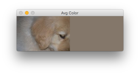
Which would give you this:

Visually, that resulting average tan looks like it would represent the puppy's colors. In practice though, you probably won't find any pixels in the puppy that match that exact shade. Even if you looked at a range of shades lighter to darker than that average, only a few of his pixels would be included. It's even likely you'd get a few pixels of his toy. As bad as the average works with the puppy, the average would totally fail on a multi-colored object, for example the FIRST® logo.

FIRST®, the FIRST® logo, FIRST® Robotics Competition (formerly also known as FRC®), FIRST® Tech Challenge (formerly also known as FTC®) are trademarks of For Inspiration and Recognition of Science and Technology (FIRST®).
K-means clustering
Let's try a more powerful method. We'll find the most common colors in our image using k-means clustering. A formal definition would go something like "k-means clustering partitions n observations into k clusters". In our case, we have a bunch of pixels (our n) and we want to pull out some number (the k) of colors.
With k-means, you have to specify the number of clusters up-front. There are other techniques that don't have this requirement. In any case, it's not a significant limitation for our needs here.
We'll use the scikit-learn library's sklearn.cluster.kmeans function to do the heavy lifting. (OpenCV itself offers a kmeans() function, but scikit's is a bit more flexible for our needs). The following script is based on a post on the PyImageSearch blog (a great resource!)
1 2 3 4 5 6 7 8 9 10 11 12 13 14 15 16 17 18 19 20 21 22 23 24 25 26 27 28 29 30 31 32 33 34 35 36 37 38 39 40 41 42 43 44 45 46 47 48 49 50 51 52 53 54 55 56 57 58 59 60 61 62 63 64 65 66 67 68 69 70 71 72 73 74 75 76 77 78 79 80 81 82 83 84 85 86 87 | |
That's a bunch of code I realize. This script does a few things; let's go through it. Skip the functions for now and jump to the "Start Here" part. The script reads in our image and determines its height and width. Then we convert it from a height by width matrix into a list of RBG values for easier processing.
Next, the script examines the image (our cropped puppy) and uses KMeans() to find the five most common colors (lines 59 - 61). The make_histogram() function essentially counts the pixels in each of those "buckets" returning those counts as a value between 0 and 1. We sort those "buckets" into a descending order of most to least common. Finally, starting on line 70, the code outputs some useful info about those dominant colors. We loop through our "buckets" to create images (aka "bars") from those colors and show them in OpenCV windows.
Output
Check out your console: the script outputs the RGB and HSV color values for each of the colored boxes.
> python dominant_color.py
Bar 1
  RGB values: (131, 114, 99)
  HSV values: (14, 62, 131)
Bar 2
  RGB values: (153, 133, 114)
  HSV values: (15, 65, 153)
Bar 3
  RGB values: (141, 138, 136)
  HSV values: (12, 9, 141)
Bar 4
  RGB values: (165, 156, 148)
  HSV values: (14, 26, 165)
Bar 5
  RGB values: (99, 87, 75)
  HSV values: (15, 62, 99)
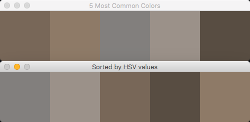
Given our cropped puppy image, the script outputs two CV2 windows. The first shows colored boxes for the top 5 dominant colors, listed most to least common left to right. If you move that window out of the way, you'll see a similar one showing those same colors arranged in HSV order (sorted lowest to highest by hue, saturation, then value).

It might be surprising when seen as RGB boxes on your screen, but the dominant colors are fairly close in hue, even in saturation. In fact, hue values range between 12 and 15. (Sidenote: OpenCV represents hue ranges from 0-180, not 0-360 as graphics apps typically do.)
This gives us just what we need to isolate objects in an image or video stream. In a future article, I'll show how to isolate objects based on their color. My plan is to then go on to show how to discern info about the object, such as its actual size, position in the real world, and so forth. But, let's not get ahead of ourselves!
In summary
In this article, I showed how to find an average color of an image. While I didn't go on to prove it with an object isolation script, average colors are typically the best way to represent a target object. Instead, I showed a more powerful technique, the k-means cluster. I showed how to determine the five most common colors. The script I provided output convenient RGB and HSV values that you can use for object isolation.
Source materials and further explorations: